
In 1990, Jeffrey Elman ran a small experiment with a tiny recurrent network.
No billion parameters.
No attention.
No massive datasets.
Just a simple question:
If a model learns to predict the next word, can it discover structure on its own?
The answer changed how we think about intelligence.
The Experiment: Learning Grammar Without Rules
Elman trained a simple recurrent network (now called an Elman network) on sentences generated from a small artificial grammar.
The setup was elegant:
- Input: one word at a time
- Objective: predict the next word
- Mechanism: feed the hidden state from time t back in at time t+1
That feedback loop meant the network carried context forward.
Time became internal state.
The training data included sentences with:
- Noun/verb distinctions
- Subject–verb agreement
- Embedded clauses (e.g., “The boy who chased the dog…”)
The network was never told what a noun or verb was.
It was never given parse trees.
Yet when Elman visualized the hidden layer representations, something striking appeared:
- Words clustered by grammatical category
- Singular and plural forms separated meaningfully
- The network tracked long-range dependencies better than expected
Structure had emerged — implicitly — from prediction.
The XOR Problem, Unfolded in Time
Before grammar, there’s a simpler way to see why recurrence matters.
The classic XOR problem is well known: given two inputs simultaneously, output 1 if exactly one is active. A single-layer perceptron can’t solve it — the decision boundary isn’t linear. Minsky and Papert proved this in 1969, and it nearly killed connectionism.
Multi-layer networks solved static XOR by adding a hidden layer. But Elman-style networks revealed something deeper: what if the two inputs don’t arrive at the same time?
Temporal XOR reformulates the problem across time steps:
- At t=1, the network sees input A
- At t=2, it sees input B
- After t=2, it must output A XOR B
The catch: by the time B arrives, A is gone. The network has no direct access to the first input anymore. It must have remembered it.
This is where the context layer earns its keep. At t=1, the hidden layer processes A and its activation is copied into the context units. At t=2, the network receives B as input and the trace of A through the context layer. It now has both — not as simultaneous inputs, but as present input combined with a compressed memory of the past.
A feedforward network cannot solve this. It has no state. Each time step is processed in isolation.
A recurrent network can, because the context units act as a form of working memory — carrying forward exactly enough information to combine with the next input.
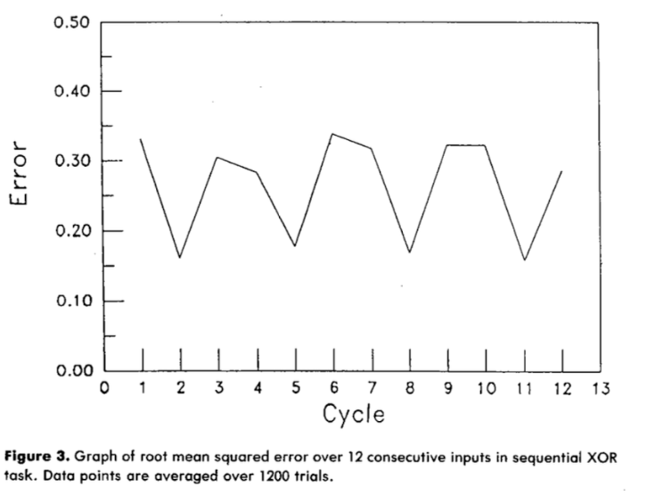
The figure above (from Elman’s 1990 paper) shows the network’s error across 12 consecutive time steps in the sequential XOR task. The zigzag pattern is the tell. Error spikes at odd-numbered cycles — when only the first input of a pair has arrived and the correct output is genuinely ambiguous. It drops at even cycles — when both inputs are available and the network can compute XOR. The network has learned where it is in the sequence. It knows when it has enough information to act and when it doesn’t. That temporal awareness, not just memory, is what recurrence buys you.
What Temporal XOR Teaches
This toy problem captures a principle that scales to every recurrent architecture:
Memory is not storage — it’s transformation. The context layer doesn’t store input A as a literal copy. It stores a transformed representation that, when combined with B, produces the right output. The network learns what to remember and how to encode it.
Time creates computational depth. Static XOR requires a hidden layer for nonlinear separation. Temporal XOR achieves the same through recurrence — unfolding in time adds the computational layers that a single-step network lacks. Recurrence trades space (more layers) for time (more steps).
Context is selective. Even in this minimal example, the network doesn’t blindly propagate everything. It learns to maintain a representation that is useful for the task. This is the seed of what LSTMs later formalize with gates — deciding what to keep, what to forget, and what to output.
Temporal XOR is the smallest possible demonstration that sequence processing is fundamentally different from static pattern matching. The moment inputs are separated by time, a system needs state. And the moment it has state, it can — in principle — learn to use it.
Elman’s grammar experiments were a far richer version of this same dynamic. Predicting the next word in “The boys who chased the dog run” requires remembering “boys” (plural) across an intervening clause. The mechanism is the same: carry forward a compressed trace, combine it with the present, and make a decision.
The Big Insight: Prediction Induces Representation
Elman’s key contribution wasn’t just recurrence.
It was this principle:
When a system must predict over time, it is forced to build internal structure.
Grammar wasn’t programmed.
It was induced by the pressure to predict accurately.
This reframed the symbolic vs. connectionist debate. Maybe rules don’t need to be explicitly stored. Maybe they are encoded in distributed state.
Humans speak grammatically without consciously applying rules.
The model behaved similarly.
Why This Still Matters
Modern large language models use the same core objective:
next-token prediction.
They don’t store grammar rules.
They don’t build explicit symbolic trees.
Yet they generate structured language, maintain coherence, and even exhibit reasoning-like behaviors.
The scale has changed.
The principle hasn’t.
We are still leveraging the same pressure:
predict the future → induce structure.
From Time to State
In Elman networks, time was literal recurrence.
Later architectures evolved:
- LSTMs introduced gating to better preserve information.
- Transformers replaced recurrence with attention.
- In transformers, “time” became encoded in positional embeddings and attention patterns.
The mechanism changed.
The philosophy deepened.
Time became state.
Instead of carrying hidden activations forward step-by-step, transformers maintain a dynamic context representation over tokens. The model still updates an internal representation conditioned on prior inputs — just without explicit recurrence.
The principle remains:
Intelligence emerges from how representations are updated across sequences.
What Comes Next
This post only scratches the surface.
In upcoming posts, I’ll explore:
- How LSTMs extended Elman’s idea with gating and memory control
- How transformers redefined temporal modeling without recurrence
- How the philosophy evolved — from “time as sequence” to “state as computation”
- And the nuances: where the analogy holds, and where it breaks
The models got bigger.
The math got sharper.
But the core idea is still beautifully simple:
If you want structure,
make a system predict through time.
References
- Elman, J. L. (1990). Finding Structure in Time. Cognitive Science, 14(2), 179–211. doi:10.1207/s15516709cog1402_1
- Elman, J. L. (1991). Distributed Representations, Simple Recurrent Networks, and Grammatical Structure. Machine Learning, 7, 195–225. doi:10.1007/BF00114844
- Minsky, M., & Papert, S. (1969). Perceptrons: An Introduction to Computational Geometry. MIT Press.